Transportation Problem
1. Application Area
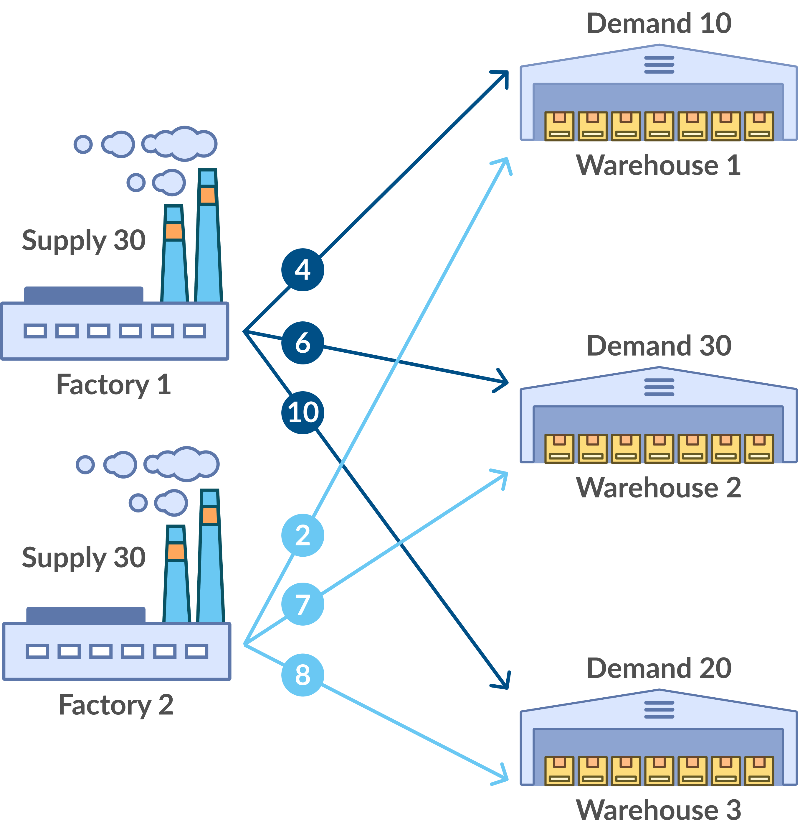
A simple transportation network is shown in Figure 1. Factories 1 and 2 are the source nodes, warehouses 1, 2 and 3 are the destination nodes, the arcs between nodes represent the existence of a path and the numbers on the arcs represent the cost of shipping each unit product through that specific path. For example, from factory 1 to warehouse 2, the cost of shipping is 6 dollars per unit. The supply and demand requirements appear beside the nodes. For example, factory 1 is capable of producing 30 units and warehouse 1 needs at least 10 units.

Figure 1: Simple transportation network
2. Genetic Algorithm
To solve the Transportation Problem using this heuristic method, the following steps are needed:
2.1. Generating the Fitness Function
The fitness function is generated by multiplying the variables in the objective function by the corresponding supply amount (highest possible value for that variable). For example, the objective function for the problem in figure 2 is:
To acquire the fitness function, we simply multiply the supply amount:
|
Destination 1 |
Destination 2 |
Destination 3 |
Supply |
|
| Source 1 | 4 | 6 | 10 | 30 |
| Source 2 | 2 | 7 | 8 | 30 |
| Demand | 10 | 30 | 20 |
Figure 2: Objective function
2.2. Creating the First Generation
The next step is to create the first generation of strings randomly. Then the strings with the lowest fitness values (since it is a minimization problem) are selected for reproduction.
2.3. Reproduction
The second generation is created by means of crossover and mutation operations. Then the best strings are chosen to create the next generation.
2.4. Checking for Feasibility
The chosen strings are checked for feasibility of solution. To be a feasible solution, the string produced has to meet all the constraints. This is checked in this step. If a string is computationally infeasible, it is rejected.
2.5. Measuring the Value of Fitness Function
When a set of feasible strings is filtered from the entire generation, their corresponding objective values are measured. For example, the string 101010 is in essence, 40(1) + 180(0) + 200(1) + 20(0) + 210(1) + 160(0) = 450.
This value (450) is then stored along with the string.
Steps 3 through 5 are then repeated for each subsequent generation of strings. After generating a sufficient number of generations, these objective values are compared and the lowest value found is declared as the optimal solution.
3. Comparison
In comparison to the existing methods, Genetic Algorithms prove to be more efficient as the size of the problem becomes greater. For a 500 x 500 problem, the heuristic method is much faster than the Simplex and Transportation Simplex Methods.
4. Conclusion
Usage of Transportation solution allows finding of optimal location for placement of warehouses, shops, or plants based on purchasing history and information about customer locations. The module provides minimization of transportation costs between locations based on algorithms of Linear Programming and suggests an optimal location for new warehouses.