Business forecasting extgended title

1. Application Area

Why is it necessary to make a Business Forecasting considering global indetermination of business processes? The answer is that all organizations operate in fuzzy conditions; however their managers should make right decisions that affect the future of their organizations. Well-founded assumptions about the future are more valuable for managers than unfounded ones. We suggest such a way of prognosis creation, which is based on logical methods to process the data generated by Microsoft Dynamics AX (Axapta).

All mentioned above does not mean that intuitive prognosis is always bad. Vice versa, ‘intrinsic’ feeling by manager often provides the only acceptable prognosis. We discuss a prognosis approach that could help responsible managers to validate their intuitive decisions. We suppose that a person, who makes decisions based on understanding of quantitative prognosis approach and who is able to use it rationally, undoubtedly has the advantage before the one, who attempts to plan the future without any additional information.

2. General Idea

Dynamics AX (Axapta) uses inventory / sales / purchase forecasting data, which are always entered by user manually, to generate planned sales and purchase orders, as well as cash flow forecast in the Ledger module. General idea of our Business Forecasting solution is to automate the creation of forecasting data based on existing historical transactions in various Dynamics AX (Axapta) modules. Supplementary idea is to take a possibility to use any Dynamics AX (Axapta) time series data for forecasting purposes. It could help users to forecast their Budgetary Analysis, Yield Projections, Process and Quality Control, Inventory Studies, Workload Projections, Utility Studies, Census Analysis, and many more.

3. Mathematical Background

Time series analysis is mathematical background of the solution.

The first step in the process of trend identification is data smoothing. The most common technique is moving average smoothing that replaces each element of the series by either the simple or weighted average of n surrounding elements, where n is the width of the smoothing "window". Seasonal dependency (seasonality) is another general component of the time series pattern. One way of evaluating the accuracy of forecasts is to plot the observed values and the one-step-ahead forecasts in identifying the residual behavior over time. Widely used statistical measures of error that can help to identify a method or the optimum value of the parameter within a method are mean absolute error and mean squared error. Mean absolute error (MAE) value is the average absolute error value. Closer this value is to zero the better the forecast is. Mean squared error (MSE) is computed as the sum (or average) of the squared error values. This is the most commonly used lack-of-fit indicator in statistical fitting procedures. As compared to the mean absolute error value, this measure is very sensitive to any outlier; that is, unique or rare large error values will impact MSE value greatly.

Technical background of the system is to use described mathematical algorithms from e.g. Matlab or Microsoft Excel. Analyzed data are exchanged between Microsoft Dynamics AX (Axapta) and computational software.

4. Forecasting Stages

The base of time-series analysis is to use data connected to past time periods to forecast future values.

Forecasting routine of this solution consists of 5 stages:

1. Selection of data from Dynamics AX (Axapta).
2. Reduction and compaction of data.
3. Building, validating, and evaluating the model.
4. Evaluation of generated prognosis and extrapolation of the model (actual prognosis).
5. Transferring the actual prognosis to Dynamics AX (Axapta).

5. Dataflow

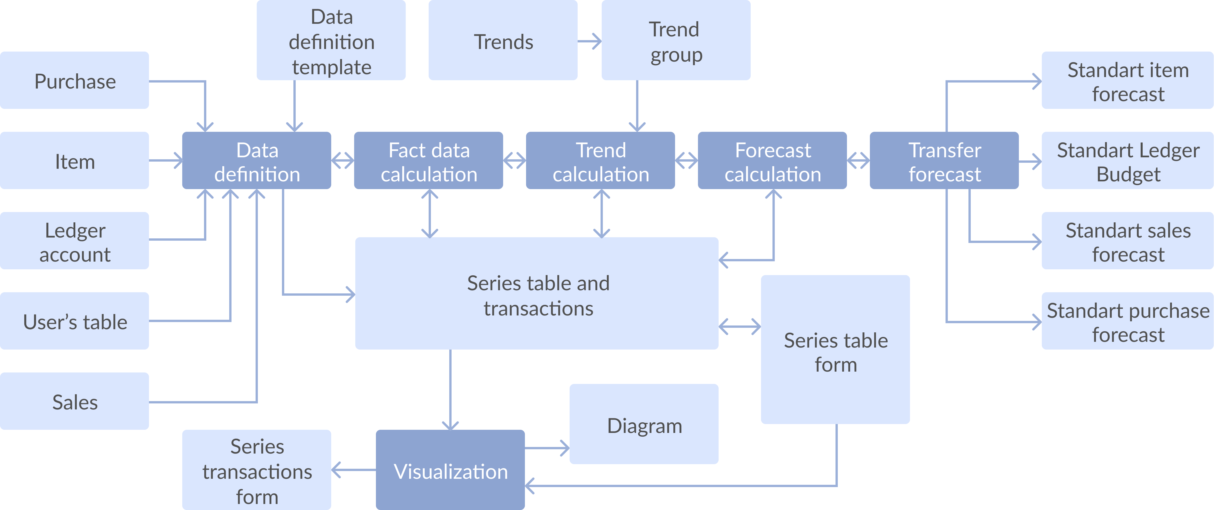
Figure 1: Dataflow diagram

6. Workflow

6.1. Data definition interface

Data definition interface allows specifying the incoming data source, the incoming data limitation query, the minimal analyzing period, the number of periods for forecast generation.

Incoming data source for forthcoming calculation

There are two possible ways for it:

• Define incoming data from predefined templates.
• Define incoming data manually by choosing necessary fields from any Dynamics AX (Axapta) table.

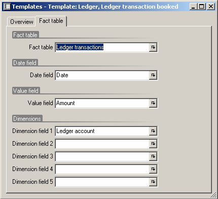
Figure 2: Template definition

Minimal analyzing period

Minimal analyzing parameter is used to define minimal date interval for building history data series and resulting forecast generation. This parameter is predefined with the following values: day, week, month, quarter, and year.

6.2. Fact data calculation

Fact data calculation normalizes incoming data series according to specified minimal analyzing period. Incoming history data are summarized by specified dimensions per each period. Resulting series are saved as fact data in data storage. This part provides noise reduction from fact table, correlation analysis in later version of calculation, and so on. User can preview a chart diagram of fetched and calculated fact data finally.

6.3. Trend line calculation

Trend line calculation routine calculates the forecasts for trends according to setup of trend group.

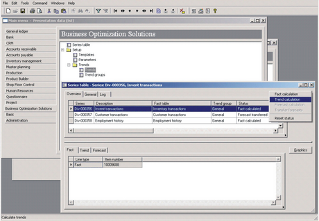
Figure 3: Trend calculation

6.4. Forecast calculation

Forecast calculation routine calculates the forecast by selected trend type.

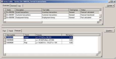
Figure 4: Forecast calculation

6.5. Store calculated data in data storage

Calculated series from fact table, startup parameters of calculation, calculated forecasts are stored in several new tables.

6.6. Visualization

Several chart diagrams are available based on pre-calculated data, trend lines data and calculated forecasts. Visualization is implemented as separate Dynamics AX (Axapta) form with Dynamics AX (Axapta) chart object utilized.

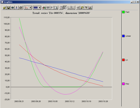
Figure 5: Visualization

6.7. Transfer calculated forecast to standard Dynamics AX (Axapta) forecast records

There is a possibility to create standard Dynamics AX (Axapta) forecast records automatically based on selected calculated forecast by trend and dimensions. Field migration rules are defined on level of startup dialog or wizard.

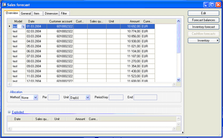
Figure 6: Transfer calculated forecast to standard Dynamics AX (Axapta) forecast records

7. Conclusion

Usage of Business Forecasting (BF) solution gains the following advantages for an enterprise:

1. BF is a base for long-term planning and budgeting.
2. BF helps in planning of production capabilities.
3. BF helps in planning of production facilities.
4. BF helps managers to validate their intuitive decisions and recognize real dependences in businesses.